3️⃣ Predicting early onset dementia - ML Modeling 🚀

The code for this series can be found here 📍
If you prefer to see the contents of the Jupyter notebook, then click here.
All the heavy-lifting has been done… now it’s time to evaluate some ML algorithms.
Evaluating ML Models⌗
The No Free Lunch theorem in Machine Learning stipulates that there is not one algorithm which works perfectly for all dataset. Thus, the performance of differing machine learning classifications will be computed and compared.
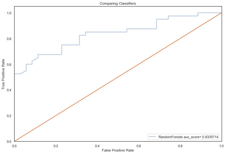
The main evaluation metric to gauge algorithm performance is the AUC (Area under ROC curve) score.
The ROC curve displays the trade-off between the true positive rate and the false positive rate.
In the case for diagnosing Dementia, it’s imperative that patients who exhibit symptoms are identified as early as possible (high true positive rate) whilst healthy patients aren’t misdiagnosed with Dementia (low false positive rate) and begin treatment.
AUC is the most appropriate performance measure as it will aid in distinguishing between the two diagnostic groups(Demented/ Nondemented).
Other evaluation metrics are used to compliment the AUC score but don’t carry the same weight. These include:
- Cross-Validation score (or gridsearch score).
- Recall score - The ratio of positive instances that each of our models detect.
- Diagnostic odds ratio (DOR score) is the odds of positivity in individuals with a illness relative to the odds in individuals without an illness.
The
evaluateAlgosfunction callsclassReportwhich computes all of the above evaluation metrics. This function will be called for a series of machine learning algos.
Before evaluation, a global scores table is defined that will record important metrics that are used to evaluate the validity of each model and whether that model is using default parameters or hyperparameters that have been tuned via grid-search or randomized grid seach:
q)scores:([models:();parameters:()]DiagnosticOddsRatio:();TrainingAccuracy:();TestAccuracy:();TestAuc:())
⚠️
A BaselineModel is used as a benchmark model. If algorithms perform better than this benchmark, it reaffirms that applying machine learning techniques to this dataset is applicable.
Please refer to the appendix for some background on each algorithm
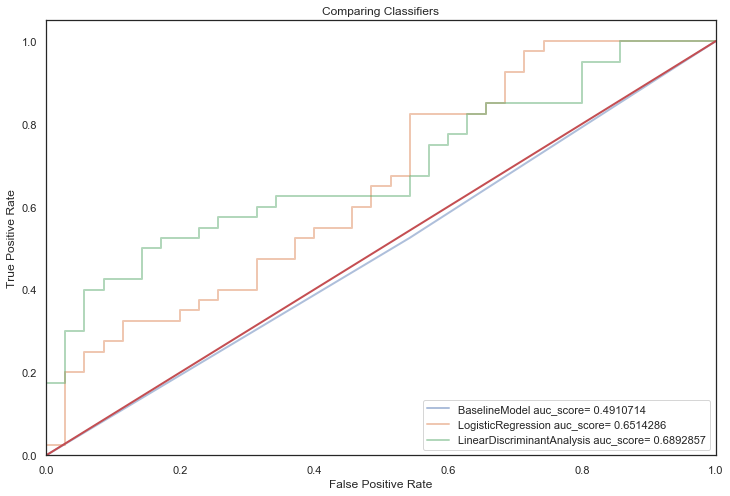
Linear classifiers are evaluated using default parameters first:
q)evaluateAlgos[linearClassifiers;`noTuning]

BaselineModel auc_score= 0.4910714

Classification report showing precision, recall and f1-score for each class:

                  precision    recall  f1-score   support

     Nondemented       0.46      0.46      0.46        35
        Demented       0.53      0.53      0.53        40

        accuracy                           0.49        75
       macro avg       0.49      0.49      0.49        75
    weighted avg       0.49      0.49      0.49        75

    DOR score: 0.9307479
    ============================================================

LogisticRegression auc_score= 0.6514286

Classification report showing precision, recall and f1-score for each class:

                  precision    recall  f1-score   support

     Nondemented       0.57      0.49      0.52        35
        Demented       0.60      0.68      0.64        40

        accuracy                           0.59        75
       macro avg       0.58      0.58      0.58        75
    weighted avg       0.58      0.59      0.58        75

    DOR score: 1.961538
    ============================================================

LinearDiscriminantAnalysis auc_score= 0.6892857

Classification report showing precision, recall and f1-score for each class:

                  precision    recall  f1-score   support

     Nondemented       0.59      0.66      0.62        35
        Demented       0.67      0.60      0.63        40

        accuracy                           0.63        75
       macro avg       0.63      0.63      0.63        75
    weighted avg       0.63      0.63      0.63        75

    DOR score: 2.875
    ============================================================
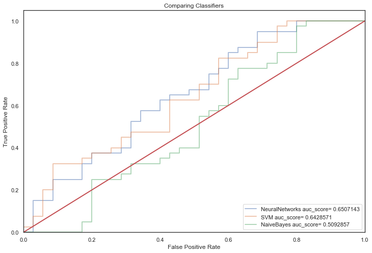
Next, non-linear classifiers with default parameters:
q)evaluateAlgos[nonLinearClassifiers;`noTuning]

NeuralNetworks auc_score= 0.6507143

Classification report showing precision, recall and f1-score for each class:

                  precision    recall  f1-score   support

     Nondemented       0.58      0.51      0.55        35
        Demented       0.61      0.68      0.64        40

        accuracy                           0.60        75
       macro avg       0.60      0.59      0.59        75
    weighted avg       0.60      0.60      0.60        75

    DOR score: 2.199095
    ============================================================

SVM auc_score= 0.6428571

Classification report showing precision, recall and f1-score for each class:

                  precision    recall  f1-score   support

     Nondemented       0.55      0.49      0.52        35
        Demented       0.59      0.65      0.62        40

        accuracy                           0.57        75
       macro avg       0.57      0.57      0.57        75
    weighted avg       0.57      0.57      0.57        75

DOR score: 1.753968
============================================================

    NaiveBayes auc_score= 0.5092857

    Classification report showing precision, recall and f1-score for each class:

                  precision    recall  f1-score   support

     Nondemented       0.54      0.20      0.29        35
        Demented       0.55      0.85      0.67        40

        accuracy                           0.55        75
       macro avg       0.54      0.53      0.48        75
    weighted avg       0.54      0.55      0.49        75

DOR score: 1.416667
============================================================
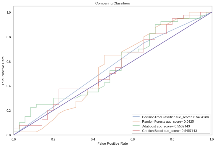
Finally, tree based classifiers:
q)evaluateAlgos[treeBasedClassifiers;`noTuning]

DecisionTreeClassifier auc_score= 0.5464286

Classification report showing precision, recall and f1-score for each class:

                  precision    recall  f1-score   support

     Nondemented       0.55      0.34      0.42        35
        Demented       0.57      0.75      0.65        40

        accuracy                           0.56        75
       macro avg       0.56      0.55      0.53        75
    weighted avg       0.56      0.56      0.54        75

DOR score: 1.565217
============================================================

RandomForests auc_score= 0.5425

Classification report showing precision, recall and f1-score for each class:

                  precision    recall  f1-score   support

     Nondemented       0.59      0.29      0.38        35
        Demented       0.57      0.82      0.67        40

        accuracy                           0.57        75
       macro avg       0.58      0.56      0.53        75
    weighted avg       0.58      0.57      0.54        75

DOR score: 1.885714
============================================================

Adaboost auc_score= 0.5532143

Classification report showing precision, recall and f1-score for each class:

                  precision    recall  f1-score   support

     Nondemented       0.67      0.29      0.40        35
        Demented       0.58      0.88      0.70        40

        accuracy                           0.60        75
       macro avg       0.62      0.58      0.55        75
    weighted avg       0.62      0.60      0.56        75

DOR score: 2.8
============================================================

GradientBoost auc_score= 0.5457143

Classification report showing precision, recall and f1-score for each class:

                  precision    recall  f1-score   support

     Nondemented       0.56      0.26      0.35        35
        Demented       0.56      0.82      0.67        40

        accuracy                           0.56        75
       macro avg       0.56      0.54      0.51        75
    weighted avg       0.56      0.56      0.52        75

DOR score: 1.631868
============================================================
q)`TestAuc xasc scores
models                     parameters| DiagnosticOddsRatio TrainingAccuracy TestAccuracy TestAuc
-------------------------------------| -----------------------------------------------------------
BaselineModel              noTuning  | 0.9307479           0.4709677        0.4933333    0.4910714
NaiveBayes                 noTuning  | 1.416667            0.7612903        0.5466667    0.5092857
RandomForests              noTuning  | 1.885714            1                0.5733333    0.5425
GradientBoost              noTuning  | 1.631868            0.9967742        0.56         0.5457143
DecisionTreeClassifier     noTuning  | 1.565217            1                0.56         0.5464286
Adaboost                   noTuning  | 2.8                 0.8903226        0.6          0.5532143
SVM                        noTuning  | 1.753968            0.7903226        0.5733333    0.6428571
NeuralNetworks             noTuning  | 2.199095            0.8677419        0.6          0.6507143
LogisticRegression         noTuning  | 1.961538            0.7967742        0.5866667    0.6514286
LinearDiscriminantAnalysis noTuning  | 2.875               0.8032258        0.6266667    0.6892857
First off, most models with default parameters provided a significant improvement over the baseline model indicating that applying Machine learning techniques to this dataset is applicable.
It is apparent that all models suffer from overfitting, a crux of having a small dataset.
They score strongly in training predictions but generalise poorly on unseen data (overfitting!).
Please refer to follow section in the appendix to see the effects of Overfitting in SVM
The next steps will try and circumvent overfitting by:
Using the Boruta Algorithm to remove irrelevant features and only retain features that fall within an area of absolute acceptance.
Using the GridSearch and RandomizedGridSearch techniques with cross validation to finely tune hyperparameters that could unknowlingly exasperate overfitting.
Part 2️⃣
Feature selection⌗
Convert the arrays back into q tables:
q)array2Tab each `X_train`X_test
X_train reverted back to q table
X_test reverted back to q table
`X_train`X_test
Feature selection is the process of finding a subset of features in the dataset X which have the greatest discriminatory power with respect to the target variable y.
If feature selection is ignored:
- It becomes computationally expensive as the model is processing a large number of features.
- garbage in, garbage out. When the number of features is significantly higher than optimal, a dip in accuracy is observed.
Occam's razorstipulates that a problem should be simplified by removing irrelevant features that would introduce unncessary noise. If a model remembers noise in a small dataset, it could generalise poorly on unseen data.
Ideally, instead of manually going through each feature to decide if any relationship exists between it and the target, an algorithm that is able to autonomously decide whether any given feature of X bears some predictive value about y is desired.
This is what the Boruta algorithm does.
The iteration count for the Boruta algorithm is arbitrary. The user provides a list of integers where:
- The iteration count is equal to the length of the list
- Each value of the list is used as a random seed value
So in the below case, 80 runs are executed against the training dataset X_train with the random seed value iterating each run (starting at 1, finishing at 80). The user decides how many features they extract from the area of acceptance (3 in this case):
q)featSelect[X_train;y_train;1+til 80;3]
Following features fell within the area of acceptance:
nwbv   | 80
mmse   | 80
educ   | 75
etiv   | 57
asf    | 55
mrDelay| 43
age    | 24
Following features fell within area of refusal/irresolution:
M      | 80
ses    | 80
visit  | 80
F      | 80
age    | 56
mrDelay| 37
asf    | 25
etiv   | 23
educ   | 5
Keeping top 3 boruta features for selection: nwbv,mmse,educ
`nwbv`mmse`educ
Reverting random seed back to 42
Important features [nwbv mmse educ] are extracted and kept using the Boruta Algorithm.
The remaining features are dropped:
q)dropCol[`X_train;cols[X_train] except borutaFeatures]
q)dropCol[`X_test;cols[X_test] except borutaFeatures]
Train and test sets are converted back to python arrays:
q)tab2Array each `X_train`X_test
X_train converted to array
X_test converted to array
Hyperparameter Tuning⌗
In order to further improve the AUC score for each model, the hyperparameters for each classifier are optimized using one of the following techniques:
- GridSearch
- RandomizedSearchCV
GridSearch simplifies the process of implementing and optimizing hyperparameters. By passing a dictionary of hyperparameters to be tested to the GridSearchCV function, all possible combinations of these values can be evaluated using cross-validation on a model selected by the user.
GridSearch is useful when the hyperparameter combinations to be explored are limited.
However, when the hyperparameter space is vast, it is better to use RandomizedSearchCV. This method operates similarly to GridSearch but with a key difference - rather than testing all possible hyperparameter combinations,
RandomizedSearchCVwill assess a fixed number of hyperparameter sets drawn from specified probability distributions. It is usually preferred over GridSearch as the user has more control over the computational resources by setting the number of iterations.
An optimalModels key table is defined that will tabulate the optimal parameters found using the grid-search/randomized grid-search technique for a particular classifier.
An optimal model will then be used by a web application to predict whether an individual is displaying alzheimer symptoms.
q)optimalModels:([mdl:()]parameters:())
A series of dictionaries are defined that represent the parameter space for each algorithm:
//Random Forest parameter space
q)rfParams:  (!) . flip(
 (`n_estimators; 15 25 30 35);
 (`min_samples_leaf; 1 + til 10);
 (`max_depth; 2 4 6);
 (`min_samples_split; 2 5 7 10 12);
 (`max_features; 2 3);
 (`criterion; `gini`entropy);
 (`class_weight; `balanced`balanced_subsample`None))

//Support vector machine parameter space
q)svcParams:(!) . flip(
 (`kernel   ; ("rbf";"linear"));
 (`C        ; 0.0001 0.001 0.01 0.1 1);
 (`degree   ; 2 3 4);
 (`gamma    ; 0.0001 0.001 0.01 0.1 0.5));

//Logistic regression parameter space
q)lrParams: (!) . flip(
 (`C        ; 0.0001 0.001 0.01 0.1 1.0 10 100);
 (`max_iter ; 1000 5000 10000 );
 (`solver;     `liblinear`lbfgs);
 (`penalty  ; ("l1";"l2")))

//Decision tree parameter space
q)dtParams: (!) . flip(
 (`max_leaf_nodes       ; 1+til 30);
 (`splitter             ; ("random";"best"));
 (`criterion            ; ("gini";"entropy"));
 (`max_depth            ; 1+til 10);
 (`min_samples_split    ; 0.1 0.2 0.3 0.5 0.6 0.7 0.8))

//Gradient Boosting parameter space
q)gbParams: (!) . flip(
 (`n_estimators      ; 500 1000 1500);
 (`learning_rate     ; 0.01 0.03 0.05 0.07);
 (`min_samples_split ; 2 4 6);
 (`min_samples_leaf  ; 3 5 7));

//Adaboost parameter space
q)adaParams: (!) . flip(
 (`n_estimators      ; 500 1000 1500 2000);
 (`learning_rate     ; 0.05 0.1 0.15 0.2))
A dictionary is defined to map each parameter space to its algorithm:
q)pspaces:(`SVM`LogisticRegression`DecisionTreeClassifier`Adaboost`GradientBoost`RandomForests)!(svcParams;lrParams;dtParams;adaParams;gbParams;rfParams)
The parameter space for each algorithm is hypertuned to compute optimal parameters:
q)f:hyperTune[;;`RandomizedSearchCV]
//Can also use the GridSearchCV optimizer to hypertune parameters - takes long, use threads (n_jobs)
//f:hyperTune[;;`GridSearchCV]
q)eachKV[f] pspaces;
============================================================
Hypertuning classifier: SVM
Best score during gridSearch is 0.7704167
Best parameter set:
kernel| "linear"
gamma | 0.5
degree| 4
C | 1f
Accuracy on training data: 0.7806452
Accuracy on test data: 0.7535714
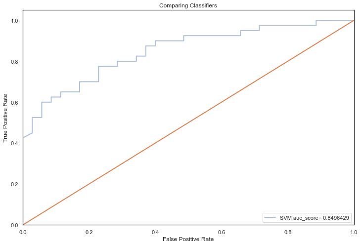
Hypertuning parameters took: 0D00:00:01.010471000
SVM auc_score= 0.8496429
Classification report showing precision, recall and f1-score for each class:
precision recall f1-score support
Nondemented 0.68 0.86 0.76 35
Demented 0.84 0.65 0.73 40
accuracy 0.75 75
macro avg 0.76 0.75 0.75 75
weighted avg 0.77 0.75 0.75 75
DOR score: 11.14286
============================================================
============================================================
Hypertuning classifier: LogisticRegression
Best score during gridSearch is 0.773125
Best parameter set:
solver | "liblinear"
penalty | "l2"
max_iter| 10000
C | 1f
Accuracy on training data: 0.7806452
Accuracy on test data: 0.7517857
Hypertuning parameters took: 0D00:00:00.360084000
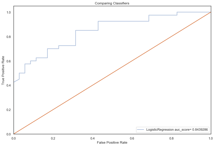
LogisticRegression auc_score= 0.8439286
Classification report showing precision, recall and f1-score for each class:
precision recall f1-score support
Nondemented 0.69 0.83 0.75 35
Demented 0.82 0.68 0.74 40
accuracy 0.75 75
macro avg 0.75 0.75 0.75 75
weighted avg 0.76 0.75 0.75 75
DOR score: 10.03846
============================================================
============================================================
Hypertuning classifier: DecisionTreeClassifier
Best score during gridSearch is 0.7452083
Best parameter set:
splitter | "random"
min_samples_split| 0.3
max_leaf_nodes | 27
max_depth | 8
criterion | "gini"
Accuracy on training data: 0.7612903
Accuracy on test data: 0.775
Hypertuning parameters took: 0D00:00:00.354700000
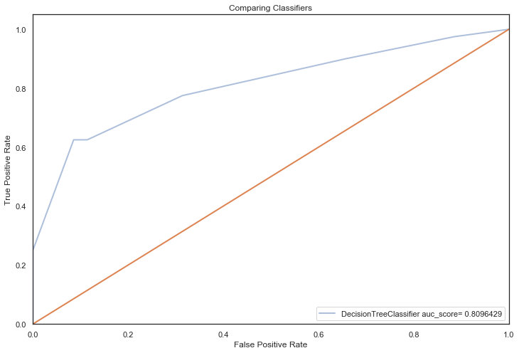
DecisionTreeClassifier auc_score= 0.8096429
Classification report showing precision, recall and f1-score for each class:
precision recall f1-score support
Nondemented 0.68 0.91 0.78 35
Demented 0.89 0.62 0.74 40
accuracy 0.76 75
macro avg 0.79 0.77 0.76 75
weighted avg 0.79 0.76 0.76 75
DOR score: 17.77778
============================================================
============================================================
Hypertuning classifier: Adaboost
Best score during gridSearch is 0.7627083
Best parameter set:
n_estimators | 500
learning_rate| 0.05
Accuracy on training data: 0.816129
Accuracy on test data: 0.7357143
Hypertuning parameters took: 0D00:04:02.047263000
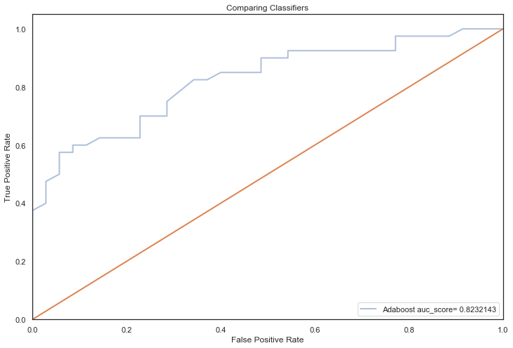
Adaboost auc_score= 0.8232143
Classification report showing precision, recall and f1-score for each class:
precision recall f1-score support
Nondemented 0.69 0.77 0.73 35
Demented 0.78 0.70 0.74 40
accuracy 0.73 75
macro avg 0.74 0.74 0.73 75
weighted avg 0.74 0.73 0.73 75
DOR score: 7.875
============================================================
============================================================
Hypertuning classifier: GradientBoost
Best score during gridSearch is 0.7604167
Best parameter set:
n_estimators | 500
min_samples_split| 4
min_samples_leaf | 7
learning_rate | 0.01
Accuracy on training data: 0.8548387
Accuracy on test data: 0.6964286
Hypertuning parameters took: 0D00:01:24.704970000
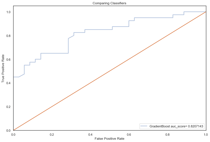
GradientBoost auc_score= 0.8207143
Classification report showing precision, recall and f1-score for each class:
precision recall f1-score support
Nondemented 0.65 0.74 0.69 35
Demented 0.74 0.65 0.69 40
accuracy 0.69 75
macro avg 0.70 0.70 0.69 75
weighted avg 0.70 0.69 0.69 75
DOR score: 5.365079
============================================================
    ============================================================

    Hypertuning classifier: RandomForests

    Best score during gridSearch is 0.756875

    Best parameter set:
    n_estimators     | 35
    min_samples_split| 10
    min_samples_leaf | 9
    max_features     | 3
    max_depth        | 4
    criterion        | "gini"
    class_weight     | "balanced"

    Accuracy on training data: 0.8032258

    Accuracy on test data: 0.7232143

    Hypertuning parameters took: 0D00:00:03.601183000
    RandomForests auc_score= 0.8335714

    Classification report showing precision, recall and f1-score for each class:

                  precision    recall  f1-score   support

     Nondemented       0.68      0.77      0.72        35
        Demented       0.77      0.68      0.72        40

        accuracy                           0.72        75
       macro avg       0.72      0.72      0.72        75
    weighted avg       0.73      0.72      0.72        75

    DOR score: 7.009615
    ============================================================
q)`TestAuc xdesc scores
models                     parameters        | DiagnosticOddsRatio TrainingAccuracy TestAccuracy TestAuc
---------------------------------------------| -----------------------------------------------------------
LogisticRegression         RandomizedSearchCV| 11.27778            0.7806452        0.76         0.8439286
SVM                        RandomizedSearchCV| 12.91667            0.7612903        0.7466667    0.8432143
DecisionTreeClassifier     RandomizedSearchCV| 7.875               0.7806452        0.7333333    0.8253571
RandomForests              RandomizedSearchCV| 7.428571            0.8322581        0.72         0.8175
Adaboost                   RandomizedSearchCV| 4.642857            0.8258065        0.68         0.7989286
GradientBoost              RandomizedSearchCV| 4.642857            0.9              0.68         0.7839286
LinearDiscriminantAnalysis noTuning          | 2.875               0.8032258        0.6266667    0.6892857
LogisticRegression         noTuning          | 1.961538            0.7967742        0.5866667    0.6514286
NeuralNetworks             noTuning          | 2.199095            0.8677419        0.6          0.6507143
SVM                        noTuning          | 1.753968            0.7903226        0.5733333    0.6428571
Adaboost                   noTuning          | 4.136364            0.8903226        0.64         0.6014286
DecisionTreeClassifier     noTuning          | 1.565217            1                0.56         0.5464286
RandomForests              noTuning          | 1.885714            1                0.5733333    0.5425
GradientBoost              noTuning          | 2.423077            0.9967742        0.5866667    0.5328571
NaiveBayes                 noTuning          | 1.416667            0.7612903        0.5466667    0.5092857
BaselineModel              noTuning          | 0.9307479           0.4709677        0.4933333    0.4910714
All models hypertuned via RandomizedGridSearchCV computed higher AUC scores than the previous no tuning evaluation, an indication that hyperparameter tuning via RandomizedSearchCV coupled with feature selection techniques, improved performance significantly (the closer to 1, the better):
q)`AucDiff xdesc select BeforeAfter:TestAuc, AucDiff: abs .[-;TestAuc] by models from scores where models in `SVM`LogisticRegression`DecisionTreeClassifier`Adaboost`GradientBoost`RandomForests
models                | BeforeAfter         AucDiff
----------------------| -----------------------------
RandomForests         | 0.5425    0.8335714 0.2910714
GradientBoost         | 0.5457143 0.8207143 0.275
Adaboost              | 0.5532143 0.8232143 0.27
DecisionTreeClassifier| 0.5464286 0.8096429 0.2632143
SVM                   | 0.6428571 0.8496429 0.2067857
LogisticRegression    | 0.6514286 0.8439286 0.1925
Conclusion⌗
The model with the highest AUC score is the SVM algo 🎉
The SVM model is relatively simple compared to boosting and ensemble algorithms, which suggest that these results support the principle of Occam’s razor, where for a small dataset, the use of straightforward models with minimal assumptions often leads to the best results.
Although, there is still some overfitting happening (training acc > test acc), mainly due to the size of this dataset, it is not as consequential as previous, as the training accuracies have decreased significantly whilst the test accuracies have risen substantially.
In essence, the models aren’t learning as many particulars in the training dataset and therefore generalising better on unseen data.
Previously, models were learning details and noise in the training data to the extent that it was generalising very poorly on unseen data.