2️⃣ Predicting early onset dementia - Data preparation 🧪

The code for this series can be found here 📍
If you prefer to see the contents of the Jupyter notebook, then click here.
Data-prep generally dominates most of a data scientist’s time during a machine-learning project.
This case is no different.
It’s very lengthyyyyyyyy 💤
I promise to try and keep this as succinct as possible but please bear with me.
Grab a ☕ and let’s get stuck into it!
Or, you can ⏭️ to the results…
Extracting numerical and categorical features⌗
Before any transformations can be applied, the training columns are split, by datatype, into their own group:
// Extract numerical, string and symbol columns
q)numCols:exec c from meta[X_train] where not t in "Cs";
q)strCols:exec c from meta[X_train] where t in "C";
q)symCols:exec c from meta[X_train] where t in "s";
Logarithmic transform⌗
As shown in the describe table some fields are highly skewed and thus have the potential to influence performance.
To circumvent this, a log-transform will be applied to each of the skewed columns (mrDelay & etiv):
q)@[`X_train;`mrDelay`etiv;{log(1+x)}]
`X_train
Categorical encoding⌗
A pivot table is computed to encode the categorical state variables - Converted,Demented and Nondemented - into binary 0 | 1 numeric values.
q)pivotTab[train_copy;`state]
state      | Converted Demented Nondemented
-----------| ------------------------------
Converted  | 1         0        0
Demented   | 0         1        0
Nondemented| 0         0        1
A left-join is then used within the dummies function to replace Converted,Demented and Nondemented values with their numeric equivalents shown in the pivot table above.
pivotTab:{[t;targ]
  prePvt:?[t;();0b;(targ,`true)!(targ;1)];
  pvtTab:0^{((union/) key each x)#/:x} ?[prePvt;();(enlist targ)!enlist targ;(lsq;targ;`true)];
  : pvtTab };

dummies:{[t;v;r]
  pvt: t lj pivotTab[t;v];
  t:(enlist v) _ pvt;
  prettyPrint t;
  @[`.;r;:;t]; };
The output is assigned to a global table aptly named dummy:
q)dummies[train_copy;`state;`dummy]
subjectId   mriId           visit mrDelay mF age educ ses mmse cdr etiv     nwbv  asf   Converted Demented Nondemented
----------------------------------------------------------------------------------------------------------------------
"OAS2_0147" "OAS2_0147_MR3" 3     1204    F  80  13   2   28   0   1336.6   0.762 1.313 0         0        1
"OAS2_0142" "OAS2_0142_MR2" 2     665     F  71  16   3   28   0   1390.443 0.81  1.262 0         0        1
"OAS2_0108" "OAS2_0108_MR2" 2     883     M  79  18   1   27   0.5 1569.498 0.781 1.118 0         1        0
"OAS2_0058" "OAS2_0058_MR1" 1     0       M  78  14   3   30   0.5 1314.52  0.707 1.335 0         1        0
"OAS2_0069" "OAS2_0069_MR2" 2     432     F  82  18   2   30   0   1470.873 0.69  1.193 0         0        1
"OAS2_0140" "OAS2_0140_MR3" 3     1655    F  81  16   3   25   0.5 1395.627 0.687 1.257 0         1        0
"OAS2_0103" "OAS2_0103_MR1" 1     0       F  69  16   1   30   0   1404.463 0.75  1.25  1         0        0
"OAS2_0086" "OAS2_0086_MR1" 1     0       F  63  15   2   28   0   1544.31  0.805 1.136 0         0        1
"OAS2_0017" "OAS2_0017_MR5" 5     2400    M  86  12   3   27   0   1813.215 0.761 0.968 0         0        1
"OAS2_0023" "OAS2_0023_MR2" 2     578     F  87  12   4   21   0.5 1249.56  0.652 1.405 0         1        0
Part 2️⃣
Correlation between features⌗
A correlation matrix is computed to gauge if any inherent relationships exist between the features and the target variable.
The target state column is converted into a dummy numeric variable to convey which attributes share the strongest correlation with it:
q)corrMatrix[dummy];
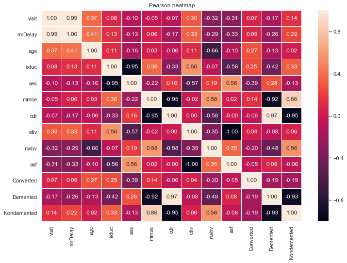
// returns a pearsons heatmap with a table detailing correlation between adjacent features
corrMatrix:{[t]
  c:exec c from meta t where t in "Cs";
  t:u cor/:\:u:c _ flip t;
  t:1!`feature xcols update feature:cols t from value t;
  : heatMap t}

//returns the x highest correlation feature_target combinations in a dataset
corrPairs:{[t;tc;n]
  c:exec c from meta[t] where t in "Cs";
  t:u cor/:\:u:c _ flip t;
  p:raze except[cols t;tc]{x,/:y except x}\:tc;
  : n#desc p!t ./: p}
The function corrPairs can also be executed to display the 5 highest +ive correlation feature pairs:
q)corrPairs[dummy;`Demented`Nondemented`Converted;5]
cdr  Demented   | 0.8327593
mmse Nondemented| 0.5301072
nwbv Nondemented| 0.316708
educ Nondemented| 0.1814134
ses  Demented   | 0.1520445
From the correlation matrix, that depicts the pearsons r (correlation coefficient) between two features, some assumptions can be hedged:
1️⃣ cdr has a strong positive correlation with Demented.
- This is expected given that the CDR scale is used to gauge whether a patient has symptoms of Dementia.
- Given that this feature is strongly correlated with the target attribute, it would be advisable to drop this column during feature selection due to collinearity.
2️⃣ age and nwbv have strong negative correlations.
3️⃣ The educ feature has strong correlations with mmse, etiv and a very strong negative correlation with ses.
4️⃣ Most of the attributes share a correlation that is close to 0 thus we assume that there is little to no linear correlation.
One-hot encoding⌗
One-hot encoding is used to transform and encode categorical values into separate binary values.
The term one-hot signifies that there is 1 hot ♨️ value in the list, whilst remaining values 0 are cold 🧊.
This is desired as most machine learning algorithms perform better when dealing with non-categorical values.
Thus, mF categorical values are encoded:
q)hotEncode[`X_train;`mF]
subjectId   mriId           visit mrDelay  age educ ses mmse cdr etiv     nwbv  asf   F M
-----------------------------------------------------------------------------------------
"OAS2_0147" "OAS2_0147_MR3" 3     7.094235 80  13   2   28   0   7.198632 0.762 1.313 1 0
"OAS2_0142" "OAS2_0142_MR2" 2     6.50129  71  16   3   28   0   7.238096 0.81  1.262 1 0
"OAS2_0108" "OAS2_0108_MR2" 2     6.784457 79  18   1   27   0.5 7.359148 0.781 1.118 0 1
"OAS2_0058" "OAS2_0058_MR1" 1     0        78  14   3   30   0.5 7.181987 0.707 1.335 0 1
"OAS2_0069" "OAS2_0069_MR2" 2     6.070738 82  18   2   30   0   7.294291 0.69  1.193 1 0
"OAS2_0140" "OAS2_0140_MR3" 3     7.41216  81  16   3   25   0.5 7.241816 0.687 1.257 1 0
"OAS2_0103" "OAS2_0103_MR1" 1     0        69  16   1   30   0   7.248122 0.75  1.25  1 0
"OAS2_0086" "OAS2_0086_MR1" 1     0        63  15   2   28   0   7.34298  0.805 1.136 1 0
"OAS2_0017" "OAS2_0017_MR5" 5     7.783641 86  12   3   27   0   7.503408 0.761 0.968 0 1
"OAS2_0023" "OAS2_0023_MR2" 2     6.361302 87  12   4   21   0.5 7.131347 0.652 1.405 1 0
..
Imputation⌗
Handling missing features within machine learning is paramount.
For various reasons, many real-world data sets come with missing values, often encoded as blanks, NaNs, or other placeholders.
Many algorithms cannot work with missing features and thus they must be dealt with.
⚠️ There’s varying options to combat this:
- 1️⃣ Delete the rows with missing features - a method only advisable when there are enough training samples in the dataset. This can introduce bias and lead to a loss of information and data 7.
- 2️⃣ Set the values to an ascertained value (mean, median or mode). This is an approximation which has the potential to add variance to the training set.
- 3️⃣ Using another machine learning algorithm to predict the missing values. This can introduce Bias and is only considered as a proxy for true values.
The function impute takes a table reference and a method (med, avg, mode) for which to infer the missing values.
Replacing missing features with the columns' median value is computed using the impute function:
q) impute[`X_train;`med]
Found nulls in the following columns: ses,mmse
Replacing nulls with the columns med value
`X_train
The values within the ses column are reversed to convey the correct information to the model.
Currently, a low ses value (1 or 2) represents a high economical status whilst a high ses value (4 or 5) depicts a low economical status.
Values are reversed ( 1->5, 2->4, 4->2, 5->1) so that the higher the score, the higher income an individual received:
q)update ses:{d:v!reverse v:asc[distinct X_train`ses];d[x]}'[ses] from `X_train
`X_train
Part 3️⃣
Detecting outliers⌗
An outlier table is defined to track any outlier values and their indices:
q)outliers:([feature:()]index:();outlier:())
The outlierDetect function uses the z-score method to detect if any datapoint has a standard score greater than a threshold value 3.
The z-score defines how many standard deviations a datapoint is away from the mean.
//Detects outliers using the z-score method
//Z score = (x -mean) / std. deviation
//t and c are the table/column where the z-score method will be executed
//r is the results table where nay outliers will be inserted
outlierDetect:{[t;c;r]
  v:t c;
  if[0< count o:where 3<=abs %[v-avg[v];dev v];
  r upsert (c;o;v o)] }

q)outlierDetect[X_train;;`outliers] each numCols;
Anamalous values are now persisted within the global outliers table:
q)outliers
feature| index                   outlier
-------| ----------------------------------------
visit  | 8 16 23 52 108 216      5 5 5 5 5 5
mmse   | 108 129 155 157 291 297 4 7 16 15 16 15f
cdr    | 157 197                 2 2f
These outliers can be visualised by graphing whiskerplots:
q)whiskerPlot select visit,mmse,cdr from X_train
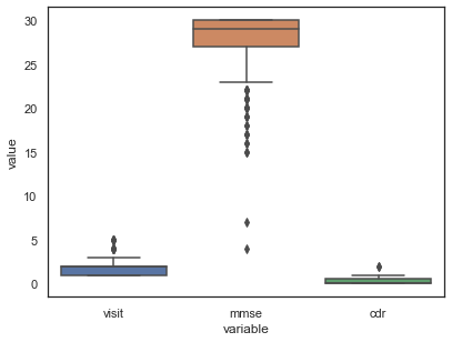
What to do with these outliers ❓
Dealing with outliers is imperative in machine learning as they can significantly influence the data and thus add extra bias during evaluation.
Some possible solutions to circumvent the effect of outliers:
1️⃣ Keep the outliers in the dataset.
- If the dataset is small,which it is in this case, it might be more costly to remove any rows as we lose information in terms of the variability in data
2️⃣ Remove the outlier rows from the training data.
3️⃣ Apply a log-transform to each outlier.
4️⃣ Clip each outlier to a given value such as the
5thor95thpercentile - a process called Winsorization
Dealing with outliers⌗
The outlierTransform function is called below, with the winsorize transform so that each outlier value is replaced with the 5th and 95th percentile respectively:
q)outlierTransform[`winsorize;`outliers]
For the visit feature, replacing outlier values:
outlier
-----------
5 5 5 5 5 5
With the winsorize value:
winsor
-----------
4 4 4 4 4 4

For the mmse feature, replacing outlier values:
outlier
---------------
4 7 16 15 16 15
With the winsorize value:
winsor
-----------------
29 29 29 29 29 29

For the cdr feature, replacing outlier values:
outlier
-------
2 2
With the winsorize value:
winsor
------
1 1
Gathering training statistics⌗
A training statistics table, trainingStats, is defined to capture important metrics of the training data.
Metrics include:
- max,min column value
- median,avg column value
- standard deviation of a column
These metrics will be used to transform unseen test data:
q)trainInfo[X_train;`trainingStats;] each  cols[X_train] except `subjectId`mriId;
q)trainingStats
feature| maxVal   minVal   medVal   avgVal    stdVal
-------| ----------------------------------------------
visit  | 4        1        2        1.855705  0.8685313
mrDelay| 7.878534 0        6.290642 4.01654   3.343527
age    | 97       60       77       76.83221  7.640762
educ   | 23       6        14       14.61074  2.900385
ses    | 5        1        4        3.57047   1.106752
mmse   | 30       17       29       27.69128  3.020954
cdr    | 1        0        0        0.2818792 0.3538956
etiv   | 7.603638 7.024444 7.296861 7.301141  0.1160262
nwbv   | 0.837    0.644    0.729    0.7300034 0.0373581
asf    | 1.563    0.876    1.19     1.19297   0.1372664
F      | 1        0        1        0.5637584 0.4959182
M      | 1        0        0        0.4362416 0.4959182
Drop irrelevant & collinear features⌗
Colinear and features are removed from the dataset:
q) dropCol[`X_train;`subjectId`mriId`cdr];
Part 4️⃣
Standardising or Normalising⌗
In machine learning it is generally a requirement that for algorithms to perform optimally, features should be standardised or normalised.
When standardising a dataset, features are rescaled so that they have the properties of a standard normal distribution with
where μ is the mean (average) and σ is the standard deviation from the mean i.e. they are centered around 0 with a std of 1 10.
The z-scores of each datapoint can then be computed using:
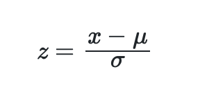
Which can be written simply in q as:
q)stdScaler:{(x-avg x) %dev x }
An alternative approach is to use normalisation (often called min-max scaling).
When using this method, data is scaled to a fixed range - usually 0 to 1. The cost of having this fixed range is that we will end up with smaller standard deviations, which can suppress the effect of outliers 10.
Min-Max scaling is performed using the following equation:
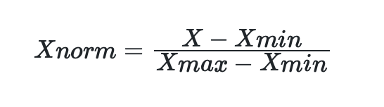
Which also can be written in q as:
q)minMaxScaler:{(x-m)%max[x]-m:min x}
There’s no obvious answer when choosing standardisation or normalisation.
Both scaling transforms are executed on the training split and their outputs are visualised below:
q)scaleBeforeAfter[stdScaler;X_train;`mmse`etiv`asf`age];
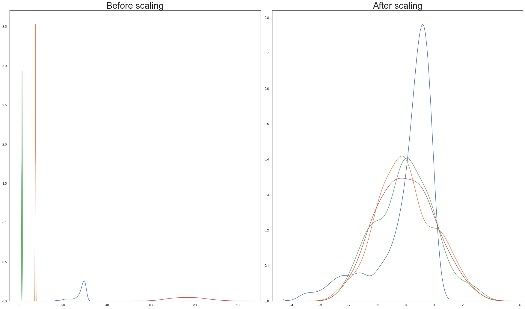
q)scaleBeforeAfter[minMaxScaler;X_train;`mmse`etiv`asf`age];
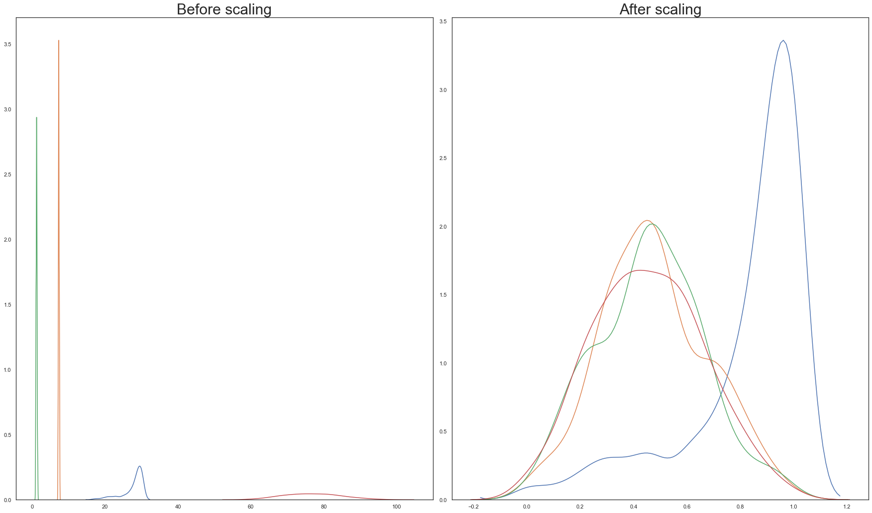
From the above graphs, Standardisation is chosen over normalisation.
This scaler is then permanently applied to the training dataset via a functional apply:
q)@[`X_train;cols X_train;stdScaler];
Next, several functions are added to the trainingStats table so that transformations can be easily reproduced on any dataset. These functions:
- perform
feature scalingby standardising or normalising numerical attributes that have different scales - perform
imputationby replacing null/missing values with a median value.
Each function is lightweight - a projection with computed training max,min,median,mean or standard deviation values.
This means transforming unseen data becomes relatively simple:
q)update stdScaler:{(x-y)%z}[;first avgVal;first stdVal],
         normaliser:{[x;minVal;maxVal] (x-minVal)%maxVal-minVal}[;first minVal;first maxVal],
         imputer:{y^x}[;first medVal] by feature from `trainingStats
For example, unseen visit values can be standardised, normalised or imputed referencing the below projections:
q)trainingStats[`visit]
maxVal    | 4f
minVal    | 1f
medVal    | 2f
avgVal    | 1.855705
stdVal    | 0.8685313
stdScaler | {(x-y)%z}[;1.855705;0.8685313]
normaliser| {[x;minVal;maxVal] (x-minVal)%maxVal-minVal}[;1f;4f]
imputer   | {y^x}[;2f]
Encode target group to numerical values⌗
Since this is a binary classification problem, the Converted values in the y_train and y_test datasets are substituted to be Demented. In addition to this, these datasets are encoded, using a vector conditional, into numerical values where:
0 = Nondemented
1 = Demented
q)update state:?[state=`Nondemented;0;1] from `y_train;
q)update state:?[state=`Nondemented;0;1] from `y_test;
After encoding the target classes, the distribution of classes in the target dataset is checked:
q)asc count'[group y_train]
state|
-----| ---
1    | 143
0    | 155
Overall, there are 12 more 0 than 1 classes.
Using a machine learning estimator out of the box when classes aren’t evenly distributed can be problematic.
To address this imbalanced class issue, new examples of the minority 1 class will be synthesised using the SMOTE technique.
Smote (Synthetic Minority Over-sampling) connects the dots between minority classes, and along these connections, creates new synthetic minority classes.
This technique is applied after the kdb+ tables are transformed into python arrays.
Shuffle training columns⌗
The order of columns are shuffled pre-evaluation:
q)X_train:shuffle[cols X_train] xcols 0!X_train;
Similar to the X_train dataset, the order of columns are shuffled pre-evaluation:
q)X_test:shuffle[cols X_test] xcols 0!X_test;
The kdb+ tables are then transformed into Python-readable matrices:
q)tab2Array each `X_train`y_train`X_test`y_test
X_train converted to array
y_train converted to array
X_test converted to array
y_test converted to array
`X_train`y_train`X_test`y_test
Note: to perform the reversal transformation i.e. a python-array to kdb+ table, run the
array2Tabfunction.
Now, as alluded to already, the class imbalanced problem is addressed using the SMOTE technique to generate some minority 1 classes:
q)sm:smote[`k_neighbors pykw 5; `random_state pykw seed]
q)`X_train`y_train set' sm[`:fit_resample][X_train;y_train]`
Finallyyyyyyyy, all feature engineering and data cleaning steps have been completed 😴
Next step, is evaluating various machine learning models and tuning their parameters to increase performance 🔥