4️⃣ Predicting early onset dementia - Creating a web GUI 🖥️

The code for this series can be found here 📍
If you prefer to see the contents of the Jupyter notebook, then click here.
This a bonus blog where we expand on the work completed in this series and build a web application which will serve as a entry-point for a potential user who wants to obtain, by entering some data fields, if they (or someone else) are exhibiting any early symptoms of dementia.
This web app will hit a kdb+ backend, which will use a ML model tuned with optimal paramaters, to predict a score between 0 and 1.
The higher the score, the greater the chance that a user exhibiting dementia.
⚠️ Note: this application does not actually predict Dementia 👇 ⚠️
It’s important to remember that the dataset used for this experiment was small, and as a result, models trained on this set, ran the risk of overfitting where models were more susceptible to seeing patterns that didn’t exist, resulting in high variance and poor generalisation on a test dataset.
Creating a web GUI to predict unseen cases⌗
Since WebSockets are supported by most modern browsers, it is possible to create a HTML5 real-time web application (GUI) and connect it to this kdb+ process through JavaScript.
A detailed introduction to websockets can be found in the Kx whitepaper Kdb+ and WebSockets: https://code.kx.com/q/wp/websockets/.
This simple GUI will serve as the entry-point for a potential client who wants to ascertain, by entering some data input, if an individual is exhibiting any symptoms of dementia.
Customising .z.ws⌗
Firstly, open some arbritary port on the q process where the ML code has been executed:
q)system"p 1992"
kdb+ has a separate message handler for WebSockets called .z.ws, meaning all incoming WebSocket messages will be processed by this function.
Note ❗
There is no default definition of
.z.ws, it has been customised (in this case) to take biomarker(mri) data and to return a result that indicates the possibility an individual is Demented (the closer to 1, the greater the confidence a subject is demented).
Breaking down each step of this custom .z.ws function:
- The query sent by the client is passed as a string for e.g.
"(\`a\`b)!(40;50)" value xsimply evaluates the string to create a dictionary.- The chosen algorithm to evaluate is extracted.
- If the
borutaoption has been enabled by the client, then every other feature, bar the significant features computed by the boruta algorithm, are dropped. If it has been disabled, all features bar[mmse educ age]are dropped. - The dictionary is then converted to a table.
- If the
- The pipeline function is called which performs a litany of feature engineering steps.
- The table is then converted to a python-like array, ready for evaluation. .
- For the chosen algorithm, the optimal parameters found through
GridSearch/RandomizedGridSearch, are used to train the algo. - The optimal model is then tested on the unseen data and returns a probability value of an individual being Nondemented / Demented.
- As all messages passed through a WebSocket connection are asynchronous, the server response is handled by
neg[.z.w]which asynchronously pushes the results back to the handle which made the request. Just before, the results are pushed back.j.jis used to convert the kdb+ output to JSON. - The client can then parse the JSON into a JavaScript object upon arrival.
q).z.ws:{
 d:value x;
 //Get classifier from dict
 clf:d[`algo];
 //If boruta is enabled, use features computed by boruta algo, if not default to only using mmse,educ and age fields
 $[`Y=d`boruta;borutaFeatures:`nwbv`mmse`educ;borutaFeatures:`mmse`educ`age];
 //Drop algo and boruta fields from dict
 d:(`algo`boruta) _ d;
 //Change to table fmt and assign it to global t table
 `t set enlist d;
 //call pipeline fn to clean the dataset
 pipeline[`t;trainingStats;cols[t] except borutaFeatures];
 //Convert to python array
 tab2Array[`t];
 //get optimal parameters for classifier
 p:optimalModels[clf;`parameters];
 //configure new model using opt params
 m:algoMappings[clf][pykwargs p];
 //fit new model with training sets
 m[`:fit][X_train;y_train];
 //predict probability of subject being demented
 pred:m[`:predict_proba][t]`;
 res: raze pred;
 //convert to json and send output back to the handle which made the request
 neg[.z.w] .j.j .Q.fmt[5;3] res 1;
 }
Using the web GUI⌗
Connect using localhost:xxxx where xxxx is the port number of the backend q process.
Hovering over the data fields will return a brief explanation:
If the handshake was successful, the web-page will return connected.
If your kdb+ application is running on an EC2 instance, connect to it using the Public DNS or Public IP of the EC2 Instance (provided firewalls/NACLs have been opened to allow incoming traffic from your IP):

Non-demented diagnosis⌗
Submitting values for an individual that has no symptoms of dementia - should return values close to 0:
Potential dementia diagnosis⌗
Submitting data values for an individual that exhibits some cognitive impairment - should return values close to 1:
Appendix⌗
Overfitting in SVM⌗
To exhibit the effects of parameter values influencing overfitting, the iris dataset, one of the most renowned machine learning datasets, is used to demonstrate tuning the hyperparameters of a support vector machine.
The hyperparameters are:
q)kernel:`linear`rbf`poly
q)C:0.01 0.1 1 10 100 1000
q)gamma:0.01 1 10 100 1000
The iris dataset is imported from sklearn’s internal datasets library:
q)datasets:.p.import[`sklearn.datasets]
q)iris:datasets[`:load_iris][]`;
q)X:iris[`data;;0 1]
q)Y:iris[`target]
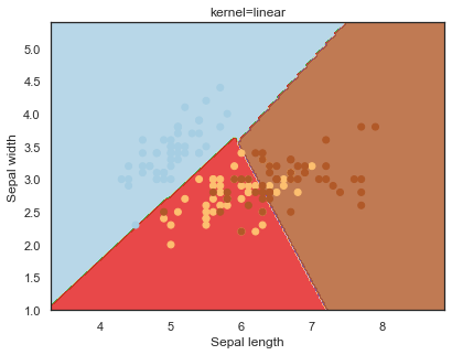
The plotSVC function allows decision boundaries in SVMs to be visualised for different parameter values:
q)plotSVC:{[title;model]
 x_min:-1+min first flip X;
 x_max:1+max first flip X;
 y_min:-1+min last flip X;
 y_max:1+max last flip X;
 h:(x_max%x_min)%100;
 x1:np[`:arange][x_min;x_max; h]`;
 y1:np[`:arange][y_min;y_max; h]`;
 b:(np[`:meshgrid][x1;y1]`);
 `xx`yy set' b;
 plt[`:subplot][1;1;1];
 z:model[`:predict][flip(raze xx;raze yy)];
 z1:164 208 # z`;
 plt[`:contourf][xx;yy;z1;`cmap pykw plt[`:cm][`:Paired];`alpha pykw 0.8];
 plt[`:scatter][X[;0]; X[;1]; `c pykw Y; `cmap pykw plt[`:cm][`:Paired]];
 plt[`:xlabel]"Sepal length";
 plt[`:ylabel]"Sepal width";
 plt[`:xlim][min first xx; max last xx];
 plt[`:title] title;
 plt[`:show][] }
An overfit function can be called to iterate over each hyperparameter value to exhibit the effects that different values have on parameters.
The parameters investigated are:
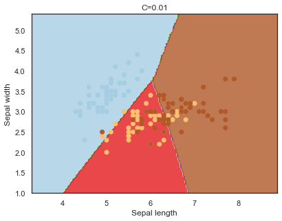
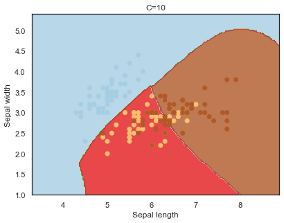
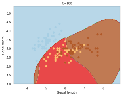
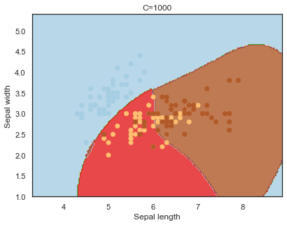
- C : the penalty for misclassifying a data point.
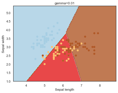
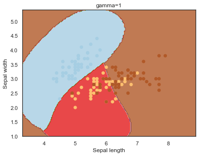
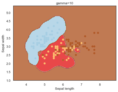
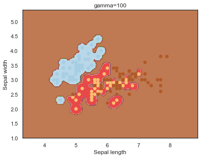
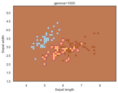
- gamma: can be thought of as the ‘spread’ of the kernel and therefore the decision region 14.
Note: The effects of C and gamma parameters are studied with a radial basis function kernel (RBF) applied to a SVM classifier.
q)overfit:{[x;y]
   title:string[x],"=",string[y];
   $[x in `gamma`C;
     mdl:svc[`kernel pykw `rbf; x pykw y][`:fit][X;Y];
     mdl:svc[x pykw y][`:fit][X;Y]];
   plotSVC[title;mdl];
 }
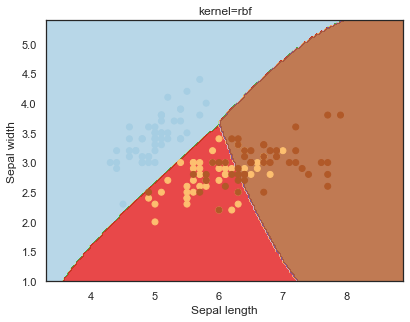
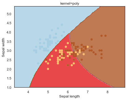
Looking at the decision boundaries for different kernels:
q)overfit[`kernel;] each kernel;
Decision boundaries for different regularization values(C):
q)overfit[`C;] each C;


Finally, comparing boundaries for different gamma values:
q)overfit[`gamma;]each gamma;